September 24, 2021

What is time?

I think I finally start to understand what is the time. If I understand correctly, time does not even exist. It is just a measure of change. Nobody cares about time, other than some living creatures. And that is because we want to be alive, to remain in our integrality or to maintain our identity. What if we don't exist? Time is there? I think not. Change is there, but not time. It looks like time is only a measurement. This is why it "flows" only forward.

September 19, 2021

Java 17 GA: Simple benchmark with Vector API (Second Preview)

A few years ago I was hoping that Java will have a chance to become again an important contented into machine learning field. I was hoping for interactivity, vectorization, and seamless integration with the external world (c/c++/fortran). With the last release of Java 17 the last two dreams are closer to reality than ever.

JEP 414: Vector API (Second Incubator) is something I awaited a lot and I spent a few hours playing with it. Personally, I am really happy with the results, and I have a lot of motivation to migrate much of the linear algebra staff on that. It looks really cool.

To make a story short, I implemented a small set of microbenchmarks for two simple operations. The first operation is fillNaN and for the second test, we simply add elements of a vector.

fillNaN

This is a common problem when working with large chunks of floating numbers: some of them are not numbers for various reasons: missing data, impossible operations, and so on. A panda version of it could be fillna. The whole idea is that for a given vector you want to replace all Double.NaN values with a given value to make arithmetic possible.

The following is a listing of the fillNa benchmark.

As you can see, nothing fancy here. The `testFillNaNArrays` method iterates over the array and if the given value is Double.NaN. Pretty straightforward. How about the results? It should be faster.

Benchmark Mode Cnt Score Error Units
VectorFillNaNBenchmark.testFillNaNArrays thrpt 10 3.405 ± 0.149 ops/ms
VectorFillNaNBenchmark.testFillNaNVectorized thrpt 10 41.930 ± 4.437 ops/ms
VectorFillNaNBenchmark.testFillNaNArrays avgt 10 0.289 ± 0.002 ms/op
VectorFillNaNBenchmark.testFillNaNVectorized avgt 10 0.023 ± 0.001 ms/op

But over 10 times faster? It is a really pleasant surprise, but not quite a surprise. This is in strict connection with auto-vectorization in Java. When it works, and for simple loops it works, it gives intrinsic optimizations and sometimes even SIMD based. But calling such a thing as Double.isNaN is not a simple thing, at least for auto-vectorization. In the new Vector API this operation is vectorized and we go fast, even if we use masks, which are not the lightest things in this new API. So we get a boost of 13x in speed which looks amazing.

sum and sumNaN

For the second microbenchmark, we have the same operation in two flavors. The first sum is implemented over all elements, with no constraints. The second sum operation, we call it sumNaN skips the potential non-numeric values and computes the sum of the rest of the numbers. We do that to check two things. We want to know how vectorization behaves compared to auto-vectorization (this is the normal sum, which is implemented as a simple loop that benefits from all optimizations possible). And we also want to see another operation with masks, compared with an auto-vectorized code. Let's see the benchmark:

And with no additional comments the results:

Benchmark Mode Cnt Score Error Units

VectorSumBenchmark.testSumArrays thrpt 10 9.264 ± 1.591 ops/ms

VectorSumBenchmark.testSumVectorized thrpt 10 12.222 ± 0.738 ops/ms

VectorSumBenchmark.testSumNanArrays thrpt 10 2.692 ± 0.191 ops/ms

VectorSumBenchmark.testSumNanVectorized thrpt 10 10.704 ± 0.428 ops/ms

VectorSumBenchmark.testSumArrays avgt 10 0.120 ± 0.011 ms/op

VectorSumBenchmark.testSumVectorized avgt 10 0.054 ± 0.011 ms/op

VectorSumBenchmark.testSumNanArrays avgt 10 0.390 ± 0.018 ms/op

VectorSumBenchmark.testSumNanVectorized avgt 10 0.068 ± 0.005 ms/op

We can see from those results that the unoptimized code for sumNan on arrays performs badly by distance. This is expected. What I personally did not expect was the vectorized version with masks (sum nan vectorized) to perform better than an auto-vectorized version of the simple sum (sum arrays). Really good job. Hat off!

Conclusions

For the sake of reproduction, I have run that on 'Intel(R) Core(TM) i7-8665U CPU @ 1.90GHz/8cores/32GB RAM'. This processor can make SIMD operations on lanes of 256 bits / 4 double floats. A better one runs faster, of course. But the absolute numbers are not important here. What is important is that you can vectorize many things in Java directly and it makes it possible to implement complex things with masks, which, at least sometimes, is faster than auto-vectorization. This is a really really amazing job.

June 7, 2016

z test in rapaio library

Hypothesis testing

(section from online manual)

Rapaio library aims to contain an extensive set of alternatives for hypothesis testing. Right now there are available just some of them. Hypothesis testing an invaluable tool to answer questions when we are dealing with uncertainty.

We deal with presenting hypothesis testing by following some examples.

Z tests

Any hypothesis test which uses normal distribution for the computed statistic is named a z test. We should note that z tests needs to know standard deviations for the involved populations. It is accustomed that when the sample is large enough the value of the population standard deviation can be estimated from data. This is not implemented in library. For the case when one does not know the involved standard deviations one can use t tests.

Note than because of this requirement, the z tests are rarely used. This is so because we rarely know the population parameters.

Example 1: One sample z-test

Sue is in charge of Quality Control at a bottling facility¹. She is checking the operation of a machine that should deliver 355 mL of liquid into an aluminum can. If the machine delivers too little, then the local Regulatory Agency may fine the company. If the machine delivers too much, then the company may lose money. For these reasons, Sue is looking for any evidence that the amount delivered by the machine is different from 355 mL.

During her investigation, Sue obtains a random sample of

10

cans. She measures the following volumes:

355.02 355.47 353.01 355.93 356.66 355.98 353.74 354.96 353.81 355.79

The machine's specifications claim that the amount of liquid delivered varies according to a normal distribution, with mean

μ

= 355 mL and standard deviation

σ

= 0.05 mL.

Do the data suggest that the machine is operating correctly?

The null hypothesis is that the machine is operating according to its specifications; thus

H_{0} : μ = 355

(

μ

is the mean volume delivered by the machine)

Sue is looking for evidence of any difference; thus, the alternate hypothesis is

H_{1} : μ \neq 355

Since the hypothesis concerns a single population mean and the population follows a normal distribution with known standard deviation, a z-test is appropriate.

What we can do is to use HTTools facility which offers shortcut methods to all implemented hypothesis tests. One of them is one sample z test which enables one to test if the sample mean is far from the expected sample mean.

// build the sample
Var cans = Numeric.copy(355.02, 355.47, 353.01, 355.93, 356.66, 355.98, 353.74, 354.96, 353.81, 355.79);
// run the test and print results
HTTools.zTestOneSample(cans, 355, 0.05).printSummary();

> HTTools.zTestOneSample

 One Sample z-test

mean: 355
sd: 0.05
significance level: 0.05
alternative hypothesis: two tails P > |z|

sample size: 10
sample mean: 355.037
z score: 2.3400855
p-value: 0.019279327322640594
conf int: [355.0060102,355.0679898]

The interpretation of the results is the following:

the z-score is $2.34$ , which means that the computed sample mean is greater with more than 2 standard deviations $2.34$
for critical level being $0.05$ and p-value $0.019$ , we reject the null hypothesis that the mean volume delivered by the machine is equal with $355$

Note: even if we know that the sample mean is greater than the proposed mean, we cannot propose this conclusion. The proper conclusion would be that is different than $355$ .

What if we ask if the machine produces more than standard specification?

We deal with this question by changing the null hypothesis. Our hypotheses become:

H_{0} : μ \leq 355

H_{1} \geq 355

Our code looks like:

HTTools.zTestOneSample(cans, 
  355, \\ mean
  0.05, \\ sd 
  0.05, \\ significance level
  HTTools.Alternative.GREATER_THAN \\ alternative
).printSummary();

> HTTools.zTestOneSample

 One Sample z-test

mean: 355
sd: 0.05
significance level: 0.05
alternative hypothesis: one tail P > z

sample size: 10
sample mean: 355.037
z score: 2.3400855
p-value: 0.009639663661320297
conf int: [355.0060102,355.0679898]

As expected the statistical power of this test is increased. As a consequence the p value was smaller and we still reject the null hypothesis. In this case we had an obvious case, when testing one side gave the same result as testing with two sides. I gave example just to help the user to pay attention to those kind of details.

1: This example is adapted from here.

Example 2: One sample z-test

A herd of $1500$ steer was fed a special high‐protein grain for a month. A random sample of $29$ were weighed and had gained an average of $6.7$ pounds. If the standard deviation of weight gain for the entire herd is $7.1$ , test the hypothesis that the average weight gain per steer for the month was more than $5$

pounds.²

We have the following null and alternative hypothesis:

H_{0} : μ = 5

H_{1} : μ > 5

ZTestOneSample ztest = HTTools.zTestOneSample(
  6.7, // sample mean
  29, // sample size
  5, // tested mean 
  7.1, // population standard deviation
  0.05, // significance level
  HTTools.Alternative.GREATER_THAN // alternative
);
ztest.printSummary();

> HTTools.zTestOneSample

 One Sample z-test

mean: 5
sd: 7.1
significance level: 0.05
alternative hypothesis: one tail P > z

sample size: 29
sample mean: 6.7
z score: 1.2894057
p-value: 0.0986285477062051
conf int: [4.1159112,9.2840888]

P-value is greater than significance level which means that we cannot reject the null hypothesis. We don't have enough evidence.

2: This example is taken from here.

Example 3: Two samples z test

The amount of a certain trace element in blood is known to vary with a standard deviation of $14.1$ ppm (parts per million) for male blood donors and $9.5$ ppm for female donors. Random samples of $75$ male and $50$ female donors yield concentration means of $28$ and $33$ ppm, respectively. What is the likelihood that the population means of concentrations of the element are the same for men and women?³

According with central limit theorem we can assume that the distribution of the sample mean is a normal distribution. More than that, since we have random samples, than the sample mean difference has a normal distribution. And because we know the standard deviation for each population, we can use a two sample z test for testing the difference of the sample means.

H_{0} : μ_{1} - μ_{2} = 0

H_{1} : μ_{1} - μ_{2} \neq 0

HTTools.zTestTwoSamples(
                28, 75, // male sample mean and size
                33, 50, // female sample mean and size
                0, // difference of means
                14.1, 9.5, // standard deviations
                ).printSummary();

> HTTools.zTestTwoSamples

 Two Samples z-test

x sample mean: 28
x sample size: 75
y sample mean: 33
y sample size: 50
mean: 0
x sd: 14.1
y sd: 9.5
significance level: 0.05
alternative hypothesis: two tails P > |z|

sample mean: -5
z score: -2.3686842
p-value: 0.017851489594360337
conf int: [-9.1372421,-0.8627579]

The test run with

0.05

significance level (because it was a default value). The alternative is two tails since we test for difference in means not equal with zero. The resulted p-value is lower than the significance value which means that we reject the hypothesis that the two populations have the same mean. We can see that also from confidence interval, since it does not include

0

Note: If we would considered a significance level of

0.01

than we would not be able to reject the null hypothesis.

3: This example is taken from here.

January 20, 2016

Tutorial on Kaggle's Titanic Competition using rapaio

I managed to finalize a Getting started guide on Kaggle's Titanic competition. This tutorial in included in the manual for the library. I tried to show some of the tools which one can find useful to participate on a machine learning competition on kaggle. The tutorial presents an easy way to get over 0.8 accuracy for this competition.

You can read the tutorial here.
The manual for rapaio library can be found here.
The code repository can be found here.

Let me know if you like it.

January 11, 2016

Rapaio Manual - Graphics: Histograms

Rapaio Manual - read online

Histogram

A histogram is a graphical representation of the distribution of a continuous variable.

The histogram is only an estimation of the distribution. To construct a histogram you have to bin the range of values from the variable in a sequence of equal length intervals, and later on counting the values from each bin. Histograms can display counts, or can display proportions which are counts divided by the total number of values.

Because the histogram uses bins that the main parameter of a histogram is the bin width. The bin's width is computed. To compute the width of a bin we need the number of bins and the minimum and maximum from the range of values. The range of values can be computed automatically from data or it can be specified when the histogram is built.

Also, the number of bins can be omitted, in which case this number is estimated also from data. For estimation is used the Freedman-Diaconis rule (see Freedman-Diaconis wikipedia page) for more details.

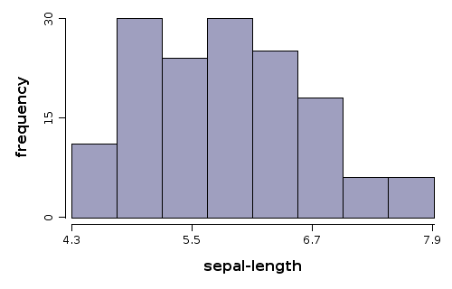
Example 1

Scope: Build a histogram with default values to estimate the pdf of sepal-length variable from iris data set.

Solution:

    WS.draw(hist(iris.var("sepal-length")));

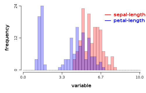
Figure 5.3.1 Histogram of `sepal-length` variable from iris data set

Example 2

Scope: Build two overlapped histograms with default values to estimate the pdf of sepal-length and petal-length variables from iris data set. We want to get bins in range (0-10) of width 0.25, colored with red, and blue, with a big transparency for visibility

Solution:

WS.draw(plot(alpha(0.3f))
    .hist(iris.var("sepal-length"), 0, 10, bins(40), color(1))
    .hist(iris.var("petal-length"), 0, 10, bins(40), color(2))
    .legend(7, 20, labels("sepal-length", "petal-length"), color(1, 2))
    .xLab("variable"));

Figure 5.3.2 Histogram of `sepal-length`, `petal-length` variable from iris data set

plot(alpha(0.3f)) - builds an empty plot; this is used only to pass default values for alpha for all plot components, otherwise the plot construct would not be needed
hist - adds a histogram to the current plot
iris.var("sepal-length") - variable used to build histogram
0, 10 - specifies the range used to compute bins
bins(40) - specifies the number of bins for histogram
color(1) - specifies the color to draw the histogram, which is the color indexed with 1 in color palette (in this case is red)
legend(7, 20, ...) - draws a legend at the specified coordinates, values are in the units specified by data
labels(..) - specifies labels for legend
color(1, 2) - specifies color for legend
xLab = specifies label text for horizontal axis